
Breast cancer is a dangerous disease for women. If it does not identify in the early-stage then the result will be the death of the patient. It is a common cancer in women worldwide. Worldwide near about 12% of women affected by breast cancer and the number is still increasing.
The doctors do not identify each and every breast cancer patient. That’s the reason Machine Learning Engineer / Data Scientist comes into the picture because they have knowledge of maths and computational power. So let’s start…….
Follow the “Breast Cancer Detection Using Machine Learning Classifier End to End Project” step by step to get 3 Bonus.
1. Raw Dataset
2. Ready to use Clean Dataset for ML project
3. Full Project in Jupyter Notebook File
- Breast Cancer Detection Machine Learning End to End Project
- Breast Cancer Detection Machine Learning Model Building
- Support Vector Classifier
- Logistic Regression
- K – Nearest Neighbor Classifier
- Naive Bayes Classifier
- Decision Tree Classifier
- Random Forest Classifier
- Adaboost Classifier
- XGBoost Classifier
- Confusion Matrix
- Classification Report of Model
- Cross-validation of the ML model
- Save the Machine Learning model
- Conclusion
Breast Cancer Detection Machine Learning End to End Project
Goal of the ML project
We have extracted features of breast cancer patient cells and normal person cells. As a Machine learning engineer / Data Scientist has to create an ML model to classify malignant and benign tumor. To complete this ML project we are using the supervised machine learning classifier algorithm.

Import essential libraries
# import libraries
import pandas as pd # for data manupulation or analysis
import numpy as np # for numeric calculation
import matplotlib.pyplot as plt # for data visualization
import seaborn as sns # for data visualization
Load breast cancer dataset & explore
We are loading breast cancer data using a scikit-learn load_brast_cancer class.
Click on the below button to download the breast cancer data in CSV file format.
#Load breast cancer dataset
from sklearn.datasets import load_breast_cancer
cancer_dataset = load_breast_cancer()
type(cancer_dataset)
Output >>> sklearn.utils.Bunch
The scikit-learn store data in an object bunch like a dictionary.
# keys in dataset
cancer_dataset.keys()
Output >>> dict_keys([‘data’, ‘target’, ‘target_names’, ‘DESCR’, ‘feature_names’, ‘filename’])
# featurs of each cells in numeric format
cancer_dataset['data']
Output >>>
array([[1.799e+01, 1.038e+01, 1.228e+02, ..., 2.654e-01, 4.601e-01,
        1.189e-01],
       [2.057e+01, 1.777e+01, 1.329e+02, ..., 1.860e-01, 2.750e-01,
        8.902e-02],
       [1.969e+01, 2.125e+01, 1.300e+02, ..., 2.430e-01, 3.613e-01,
        8.758e-02],
       ...,
       [1.660e+01, 2.808e+01, 1.083e+02, ..., 1.418e-01, 2.218e-01,
        7.820e-02],
       [2.060e+01, 2.933e+01, 1.401e+02, ..., 2.650e-01, 4.087e-01,
        1.240e-01],
       [7.760e+00, 2.454e+01, 4.792e+01, ..., 0.000e+00, 2.871e-01,
        7.039e-02]])
These numeric values are extracted features of each cell.
# malignant or benign value
cancer_dataset['target']
The target stores the values of malignant or benign tumors.
# target value name malignant or benign tumor
cancer_dataset['target_names']
Output >>> array([‘malignant’, ‘benign’], dtype='<U9′)
0 means malignant tumor
1 mean benign tumor
The cancer_dataset[‘DESCR’] store the description of breast cancer dataset.
# description of data
print(cancer_dataset['DESCR'])
Output >>>
.. _breast_cancer_dataset:

Breast cancer wisconsin (diagnostic) dataset
--------------------------------------------

**Data Set Characteristics:**
    :Number of Instances: 569
    :Number of Attributes: 30 numeric, predictive attributes and the class
    :Attribute Information:
        - radius (mean of distances from center to points on the perimeter)
        - texture (standard deviation of gray-scale values)
        - perimeter
        - area
        - smoothness (local variation in radius lengths)
        - compactness (perimeter^2 / area - 1.0)
        - concavity (severity of concave portions of the contour)
        - concave points (number of concave portions of the contour)
        - symmetry
        - fractal dimension ("coastline approximation" - 1)

        The mean, standard error, and "worst" or largest (mean of the three
        largest values) of these features were computed for each image,
        resulting in 30 features.  For instance, field 3 is Mean Radius, field
        13 is Radius SE, field 23 is Worst Radius.

        - class:
                - WDBC-Malignant
                - WDBC-Benign

    :Summary Statistics:
    ===================================== ====== ======
                                           Min    Max
    ===================================== ====== ======
    radius (mean):                        6.981  28.11
    texture (mean):                       9.71   39.28
    perimeter (mean):                     43.79  188.5
    area (mean):                          143.5  2501.0
    smoothness (mean):                    0.053  0.163
    compactness (mean):                   0.019  0.345
    concavity (mean):                     0.0    0.427
    concave points (mean):                0.0    0.201
    symmetry (mean):                      0.106  0.304
    fractal dimension (mean):             0.05   0.097
    radius (standard error):              0.112  2.873
    texture (standard error):             0.36   4.885
    perimeter (standard error):           0.757  21.98
    area (standard error):                6.802  542.2
    smoothness (standard error):          0.002  0.031
    compactness (standard error):         0.002  0.135
    concavity (standard error):           0.0    0.396
    concave points (standard error):      0.0    0.053
    symmetry (standard error):            0.008  0.079
    fractal dimension (standard error):   0.001  0.03
    radius (worst):                       7.93   36.04
    texture (worst):                      12.02  49.54
    perimeter (worst):                    50.41  251.2
    area (worst):                         185.2  4254.0
    smoothness (worst):                   0.071  0.223
    compactness (worst):                  0.027  1.058
    concavity (worst):                    0.0    1.252
    concave points (worst):               0.0    0.291
    symmetry (worst):                     0.156  0.664
    fractal dimension (worst):            0.055  0.208
    ===================================== ====== ======

    :Missing Attribute Values: None
    :Class Distribution: 212 - Malignant, 357 - Benign
    :Creator:  Dr. William H. Wolberg, W. Nick Street, Olvi L. Mangasarian
    :Donor: Nick Street
    :Date: November, 1995

This is a copy of UCI ML Breast Cancer Wisconsin (Diagnostic) datasets.
https://goo.gl/U2Uwz2

Features are computed from a digitized image of a fine needle
aspirate (FNA) of a breast mass.  They describe
characteristics of the cell nuclei present in the image.

Separating plane described above was obtained using
Multisurface Method-Tree (MSM-T) [K. P. Bennett, "Decision Tree
Construction Via Linear Programming." Proceedings of the 4th
Midwest Artificial Intelligence and Cognitive Science Society,
pp. 97-101, 1992], a classification method which uses linear
programming to construct a decision tree.  Relevant features
were selected using an exhaustive search in the space of 1-4
features and 1-3 separating planes.

The actual linear program used to obtain the separating plane
in the 3-dimensional space is that described in:
[K. P. Bennett and O. L. Mangasarian: "Robust Linear
Programming Discrimination of Two Linearly Inseparable Sets",
Optimization Methods and Software 1, 1992, 23-34].

This database is also available through the UW CS ftp server:

ftp ftp.cs.wisc.edu
cd math-prog/cpo-dataset/machine-learn/WDBC/

.. topic:: References

   - W.N. Street, W.H. Wolberg and O.L. Mangasarian. Nuclear feature extraction
     for breast tumor diagnosis. IS&T/SPIE 1993 International Symposium on
     Electronic Imaging: Science and Technology, volume 1905, pages 861-870,
     San Jose, CA, 1993.
   - O.L. Mangasarian, W.N. Street and W.H. Wolberg. Breast cancer diagnosis and
     prognosis via linear programming. Operations Research, 43(4), pages 570-577,
     July-August 1995.
   - W.H. Wolberg, W.N. Street, and O.L. Mangasarian. Machine learning techniques
     to diagnose breast cancer from fine-needle aspirates. Cancer Letters 77 (1994)
     163-171.
Features name of malignant & benign tumor.
# name of features
print(cancer_dataset['feature_names'])
Output >>>
['mean radius' 'mean texture' 'mean perimeter' 'mean area'
 'mean smoothness' 'mean compactness' 'mean concavity'
 'mean concave points' 'mean symmetry' 'mean fractal dimension'
 'radius error' 'texture error' 'perimeter error' 'area error'
 'smoothness error' 'compactness error' 'concavity error'
 'concave points error' 'symmetry error' 'fractal dimension error'
 'worst radius' 'worst texture' 'worst perimeter' 'worst area'
 'worst smoothness' 'worst compactness' 'worst concavity'
 'worst concave points' 'worst symmetry' 'worst fractal dimension']
When we call load_breast_cancer() class it downloads breast_cancer.csv file and you can see file location.
# location/path of data file
print(cancer_dataset['filename'])
Output >>> C:\ProgramData\Anaconda3\lib\site-packages\sklearn\datasets\data\breast_cancer.csv
Create DataFrame
Now, we are creating DataFrame by concate ‘data’ and ‘target’ together and give columns name.
# create datafrmae
cancer_df = pd.DataFrame(np.c_[cancer_dataset['data'],cancer_dataset['target']],
             columns = np.append(cancer_dataset['feature_names'], ['target']))
Click on the below button to download breast cancer DataFrame in CSV file format.
Head of cancer DataFrame
# Head of cancer DataFrame
cancer_df.head(6)
Output >>>

The tail of cancer DataFrame
# Tail of cancer DataFrame
cancer_df.tail(6)
Output >>>

Getting information of cancer DataFrame using ‘.info()‘ method.
# Information of cancer Dataframe
cancer_df.info()
Output >>>
<class 'pandas.core.frame.DataFrame'>
RangeIndex: 569 entries, 0 to 568
Data columns (total 31 columns):
mean radius                569 non-null float64
mean texture               569 non-null float64
mean perimeter             569 non-null float64
mean area                  569 non-null float64
mean smoothness            569 non-null float64
mean compactness           569 non-null float64
mean concavity             569 non-null float64
mean concave points        569 non-null float64
mean symmetry              569 non-null float64
mean fractal dimension     569 non-null float64
radius error               569 non-null float64
texture error              569 non-null float64
perimeter error            569 non-null float64
area error                 569 non-null float64
smoothness error           569 non-null float64
compactness error          569 non-null float64
concavity error            569 non-null float64
concave points error       569 non-null float64
symmetry error             569 non-null float64
fractal dimension error    569 non-null float64
worst radius               569 non-null float64
worst texture              569 non-null float64
worst perimeter            569 non-null float64
worst area                 569 non-null float64
worst smoothness           569 non-null float64
worst compactness          569 non-null float64
worst concavity            569 non-null float64
worst concave points       569 non-null float64
worst symmetry             569 non-null float64
worst fractal dimension    569 non-null float64
target                     569 non-null float64
dtypes: float64(31)
memory usage: 137.9 KB
We have a total of non-null 569 patients’ information with 31 features. All feature data types in the float. The size of the DataFrame is 137.9 KB.
Numerical distribution of data. We can know to mean, standard deviation, min, max, 25%,50% and 75% value of each feature.
# Numerical distribution of data
cancer_df.describe()
Output >>>

We have clean and well formated DataFrame, so DtaFrame is ready to visualize.
Data Visualization
Pair plot of breast cancer data
Basically, the pair plot is used to show the numeric distribution in the scatter plot.
# Paiplot of cancer dataframe
sns.pairplot(cancer_df, hue = 'target')
Output >>>

Pair plot of sample feature of DataFrame
# pair plot of sample feature
sns.pairplot(cancer_df, hue = 'target',
             vars = ['mean radius', 'mean texture', 'mean perimeter', 'mean area', 'mean smoothness'] )
Output >>>

The pair plot showing malignant and benign tumor data distributed in two classes. It is easy to differentiate in the pair plot.
Counterplot
Showing the total count of malignant and benign tumor patients in counterplot.
# Count the target class
sns.countplot(cancer_df['target'])
Output >>>

In the below counterplot max samples mean radius is equal to 1.
# counter plot of feature mean radius
plt.figure(figsize = (20,8))
sns.countplot(cancer_df['mean radius'])

Heatmap
Heatmap of breast cancer DataFrame
In the below heatmap we can see the variety of different feature’s value. The value of feature ‘mean area’ and ‘worst area’ are greater than other and ‘mean perimeter’, ‘area error’, and ‘worst perimeter’ value slightly less but greater than remaining features.
# heatmap of DataFrame
plt.figure(figsize=(16,9))
sns.heatmap(cancer_df)
Output >>>

Heatmap of a correlation matrix
To find a correlation between each feature and target we visualize heatmap using the correlation matrix.
# Heatmap of Correlation matrix of breast cancer DataFrame
plt.figure(figsize=(20,20))
sns.heatmap(cancer_df.corr(), annot = True, cmap ='coolwarm', linewidths=2)
Output >>>

Correlation barplot
Taking the correlation of each feature with the target and the visualize barplot.
# create second DataFrame by droping target
cancer_df2 = cancer_df.drop(['target'], axis = 1)
print("The shape of 'cancer_df2' is : ", cancer_df2.shape)
Output >>> The shape of ‘cancer_df2’ is : (569, 30)
# visualize correlation barplot
plt.figure(figsize = (16,5))
ax = sns.barplot(cancer_df2.corrwith(cancer_df.target).index, cancer_df2.corrwith(cancer_df.target))
ax.tick_params(labelrotation = 90)
Output >>>

In the above correlation barplot only feature ‘smoothness error’ is strongly positively correlated with the target than others. The features ‘mean factor dimension’, ‘texture error’, and ‘symmetry error’ are very less positive correlated and others remaining are strongly negatively correlated.
Data Preprocessing
Split DataFrame in train and test
# input variable
X = cancer_df.drop(['target'], axis = 1)
X.head(6)
Output >>>

# output variable
y = cancer_df['target']
y.head(6)
Output >>>
0    0.0
1    0.0
2    0.0
3    0.0
4    0.0
5    0.0
Name: target, dtype: float64
# split dataset into train and test
from sklearn.model_selection import train_test_split
X_train, X_test, y_train, y_test = train_test_split(X, y, test_size = 0.2, random_state= 5)
Feature Scaling
Converting different units and magnitude data in one unit.
# Feature scaling
from sklearn.preprocessing import StandardScaler
sc = StandardScaler()
X_train_sc = sc.fit_transform(X_train)
X_test_sc = sc.transform(X_test)
Breast Cancer Detection Machine Learning Model Building
We have clean data to build the Ml model. But which Machine learning algorithm is best for the data we have to find. The output is a categorical format so we will use supervised classification machine learning algorithms.
To build the best model, we have to train and test the dataset with multiple Machine Learning algorithms then we can find the best ML model. So let’s try.
First, we need to import the required packages.
from sklearn.metrics import confusion_matrix, classification_report, accuracy_score
Support Vector Classifier
# Support vector classifier
from sklearn.svm import SVC
svc_classifier = SVC()
svc_classifier.fit(X_train, y_train)
y_pred_scv = svc_classifier.predict(X_test)
accuracy_score(y_test, y_pred_scv)
Output >>> 0.5789473684210527
# Train with Standard scaled Data
svc_classifier2 = SVC()
svc_classifier2.fit(X_train_sc, y_train)
y_pred_svc_sc = svc_classifier2.predict(X_test_sc)
accuracy_score(y_test, y_pred_svc_sc)
Output >>> 0.9649122807017544
Logistic Regression
# Logistic Regression
from sklearn.linear_model import LogisticRegression
lr_classifier = LogisticRegression(random_state = 51, penalty = 'l1')
lr_classifier.fit(X_train, y_train)
y_pred_lr = lr_classifier.predict(X_test)
accuracy_score(y_test, y_pred_lr)
Output >>> 0.9736842105263158
# Train with Standard scaled Data
lr_classifier2 = LogisticRegression(random_state = 51, penalty = 'l1')
lr_classifier2.fit(X_train_sc, y_train)
y_pred_lr_sc = lr_classifier.predict(X_test_sc)
accuracy_score(y_test, y_pred_lr_sc)
Output >>> 0.5526315789473685
K – Nearest Neighbor Classifier
# K – Nearest Neighbor Classifier
from sklearn.neighbors import KNeighborsClassifier
knn_classifier = KNeighborsClassifier(n_neighbors = 5, metric = 'minkowski', p = 2)
knn_classifier.fit(X_train, y_train)
y_pred_knn = knn_classifier.predict(X_test)
accuracy_score(y_test, y_pred_knn)
Output >>> 0.9385964912280702
# Train with Standard scaled Data
knn_classifier2 = KNeighborsClassifier(n_neighbors = 5, metric = 'minkowski', p = 2)
knn_classifier2.fit(X_train_sc, y_train)
y_pred_knn_sc = knn_classifier.predict(X_test_sc)
accuracy_score(y_test, y_pred_knn_sc)
Output >>> 0.5789473684210527
Naive Bayes Classifier
# Naive Bayes Classifier
from sklearn.naive_bayes import GaussianNB
nb_classifier = GaussianNB()
nb_classifier.fit(X_train, y_train)
y_pred_nb = nb_classifier.predict(X_test)
accuracy_score(y_test, y_pred_nb)
Output >>> 0.9473684210526315
# Train with Standard scaled Data
nb_classifier2 = GaussianNB()
nb_classifier2.fit(X_train_sc, y_train)
y_pred_nb_sc = nb_classifier2.predict(X_test_sc)
accuracy_score(y_test, y_pred_nb_sc)
Output >>> 0.9385964912280702
Decision Tree Classifier
# Decision Tree Classifier
from sklearn.tree import DecisionTreeClassifier
dt_classifier = DecisionTreeClassifier(criterion = 'entropy', random_state = 51)
dt_classifier.fit(X_train, y_train)
y_pred_dt = dt_classifier.predict(X_test)
accuracy_score(y_test, y_pred_dt)
Output >>> 0.9473684210526315
# Train with Standard scaled Data
dt_classifier2 = DecisionTreeClassifier(criterion = 'entropy', random_state = 51)
dt_classifier2.fit(X_train_sc, y_train)
y_pred_dt_sc = dt_classifier.predict(X_test_sc)
accuracy_score(y_test, y_pred_dt_sc)
Output >>> 0.7543859649122807
Random Forest Classifier
# Random Forest Classifier
from sklearn.ensemble import RandomForestClassifier
rf_classifier = RandomForestClassifier(n_estimators = 20, criterion = 'entropy', random_state = 51)
rf_classifier.fit(X_train, y_train)
y_pred_rf = rf_classifier.predict(X_test)
accuracy_score(y_test, y_pred_rf)
Output >>> 0.9736842105263158
# Train with Standard scaled Data
rf_classifier2 = RandomForestClassifier(n_estimators = 20, criterion = 'entropy', random_state = 51)
rf_classifier2.fit(X_train_sc, y_train)
y_pred_rf_sc = rf_classifier.predict(X_test_sc)
accuracy_score(y_test, y_pred_rf_sc)
Output >>> 0.7543859649122807
Adaboost Classifier
# Adaboost Classifier
from sklearn.ensemble import AdaBoostClassifier
adb_classifier = AdaBoostClassifier(DecisionTreeClassifier(criterion = 'entropy', random_state = 200),
                                    n_estimators=2000,
                                    learning_rate=0.1,
                                    algorithm='SAMME.R',
                                    random_state=1,)
adb_classifier.fit(X_train, y_train)
y_pred_adb = adb_classifier.predict(X_test)
accuracy_score(y_test, y_pred_adb)
Output >>> 0.9473684210526315
# Train with Standard scaled Data
adb_classifier2 = AdaBoostClassifier(DecisionTreeClassifier(criterion = 'entropy', random_state = 200),
                                    n_estimators=2000,
                                    learning_rate=0.1,
                                    algorithm='SAMME.R',
                                    random_state=1,)
adb_classifier2.fit(X_train_sc, y_train)
y_pred_adb_sc = adb_classifier2.predict(X_test_sc)
accuracy_score(y_test, y_pred_adb_sc)
Output >>> 0.9473684210526315
XGBoost Classifier
# XGBoost Classifier
from xgboost import XGBClassifier
xgb_classifier = XGBClassifier()
xgb_classifier.fit(X_train, y_train)
y_pred_xgb = xgb_classifier.predict(X_test)
accuracy_score(y_test, y_pred_xgb)
Output >>> 0.9824561403508771
# Train with Standard scaled Data
xgb_classifier2 = XGBClassifier()
xgb_classifier2.fit(X_train_sc, y_train)
y_pred_xgb_sc = xgb_classifier2.predict(X_test_sc)
accuracy_score(y_test, y_pred_xgb_sc)
Output >>> 0.9824561403508771
XGBoost Parameter Tuning Randomized Search
# XGBoost classifier most required parameters
params={
 "learning_rate"    : [0.05, 0.10, 0.15, 0.20, 0.25, 0.30 ] ,
 "max_depth"        : [ 3, 4, 5, 6, 8, 10, 12, 15],
 "min_child_weight" : [ 1, 3, 5, 7 ],
 "gamma"            : [ 0.0, 0.1, 0.2 , 0.3, 0.4 ],
 "colsample_bytree" : [ 0.3, 0.4, 0.5 , 0.7 ]
}
# Randomized Search
from sklearn.model_selection import RandomizedSearchCV
random_search = RandomizedSearchCV(xgb_classifier, param_distributions=params, scoring= 'roc_auc', n_jobs= -1, verbose= 3)
random_search.fit(X_train, y_train)
Output >>>
RandomizedSearchCV(cv='warn', error_score='raise-deprecating',
          estimator=XGBClassifier(base_score=0.5, booster='gbtree', colsample_bylevel=1,
       colsample_bynode=1, colsample_bytree=1, gamma=0, learning_rate=0.1,
       max_delta_step=0, max_depth=3, min_child_weight=1, missing=None,
       n_estimators=100, n_jobs=1, nthread=None,
       objective='binary:logistic', random_state=0, reg_alpha=0,
       reg_lambda=1, scale_pos_weight=1, seed=None, silent=None,
       subsample=1, verbosity=1),
          fit_params=None, iid='warn', n_iter=10, n_jobs=-1,
          param_distributions={'learning_rate': [0.05, 0.1, 0.15, 0.2, 0.25, 0.3], 'max_depth': [3, 4, 5, 6, 8, 10, 12, 15], 'min_child_weight': [1, 3, 5, 7], 'gamma': [0.0, 0.1, 0.2, 0.3, 0.4], 'colsample_bytree': [0.3, 0.4, 0.5, 0.7]},
          pre_dispatch='2*n_jobs', random_state=None, refit=True,
          return_train_score='warn', scoring='roc_auc', verbose=3)
random_search.best_params_
Output >>>
{'min_child_weight': 1,
 'max_depth': 3,
 'learning_rate': 0.3,
 'gamma': 0.4,
 'colsample_bytree': 0.3}
random_search.best_estimator_
Output >>>
XGBClassifier(base_score=0.5, booster='gbtree', colsample_bylevel=1,
       colsample_bynode=1, colsample_bytree=0.3, gamma=0.4,
       learning_rate=0.3, max_delta_step=0, max_depth=3,
       min_child_weight=1, missing=None, n_estimators=100, n_jobs=1,
       nthread=None, objective='binary:logistic', random_state=0,
       reg_alpha=0, reg_lambda=1, scale_pos_weight=1, seed=None,
       silent=None, subsample=1, verbosity=1)
# training XGBoost classifier with best parameters
xgb_classifier_pt = XGBClassifier(base_score=0.5, booster='gbtree', colsample_bylevel=1,
       colsample_bynode=1, colsample_bytree=0.4, gamma=0.2,
       learning_rate=0.1, max_delta_step=0, max_depth=15,
       min_child_weight=1, missing=None, n_estimators=100, n_jobs=1,
       nthread=None, objective='binary:logistic', random_state=0,
       reg_alpha=0, reg_lambda=1, scale_pos_weight=1, seed=None,
       silent=None, subsample=1, verbosity=1)

xgb_classifier_pt.fit(X_train, y_train)
y_pred_xgb_pt = xgb_classifier_pt.predict(X_test)
accuracy_score(y_test, y_pred_xgb_pt)
Output >>> 0.9824561403508771
Confusion Matrix
cm = confusion_matrix(y_test, y_pred_xgb_pt)
plt.title('Heatmap of Confusion Matrix', fontsize = 15)
sns.heatmap(cm, annot = True)
plt.show()
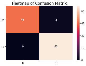
The model is giving 0% type II error and it is best.
Classification Report of Model
print(classification_report(y_test, y_pred_xgb_pt))
Output >>>
              precision    recall  f1-score   support

         0.0       1.00      0.96      0.98        48
         1.0       0.97      1.00      0.99        66

   micro avg       0.98      0.98      0.98       114
   macro avg       0.99      0.98      0.98       114
weighted avg       0.98      0.98      0.98       114
Cross-validation of the ML model
To find the ML model is overfitted, under fitted or generalize doing cross-validation.
# Cross validation
from sklearn.model_selection import cross_val_score
cross_validation = cross_val_score(estimator = xgb_model_pt2, X = X_train_sc, y = y_train, cv = 10)
print("Cross validation of XGBoost model = ",cross_validation)
print("Cross validation of XGBoost model (in mean) = ",cross_validation.mean())
from sklearn.model_selection import cross_val_score
cross_validation = cross_val_score(estimator = xgb_classifier_pt, X = X_train_sc,y = y_train, cv = 10)
print("Cross validation accuracy of XGBoost model = ", cross_validation)
print("\nCross validation mean accuracy of XGBoost model = ", cross_validation.mean())
Output >>>
Cross validation accuracy of XGBoost model =  [0.9787234  0.97826087 0.97826087 0.97826087 0.93333333 0.91111111
 1.         1.         0.97777778 0.88888889]

Cross validation mean accuracy of XGBoost model =  0.9624617124062083
The mean accuracy value of cross-validation is 96.24% and XGBoost model accuracy is 98.24%. It showing XGBoost is slightly overfitted but when training data will more it will generalized model.
Save the Machine Learning model
After completion of the Machine Learning project or building the ML model need to deploy in an application. To deploy the ML model need to save it first. To save the Machine Learning project we can use the pickle or joblib package.
Here, we will use pickle, Use anyone which is better for you.
## Pickle
import pickle

# save model
pickle.dump(xgb_classifier_pt, open('breast_cancer_detector.pickle', 'wb'))

# load model
breast_cancer_detector_model = pickle.load(open('breast_cancer_detector.pickle', 'rb'))

# predict the output
y_pred = breast_cancer_detector_model.predict(X_test)

# confusion matrix
print('Confusion matrix of XGBoost model: \n',confusion_matrix(y_test, y_pred),'\n')

# show the accuracy
print('Accuracy of XGBoost model = ',accuracy_score(y_test, y_pred))
Output >>>
Confusion matrix of XGBoost model:
 [[46  2]
 [ 0 66]]

Accuracy of XGBoost model =  0.9824561403508771
Note: When we dump the model then model file is store in the disk where the project file is store but we can change path by passing its address.
Congratulation!!!!!!!
We have completed the Machine learning Project successfully with 98.24% accuracy which is great for ‘Breast Cancer Detection using Machine learning’ project. Now, we are ready to deploy our ML model in the healthcare project.
Click on the below button to download the ‘ Breast Cancer Detection ‘ Machine Learning end to end project in the Jupyter Notebook file.
Conclusion
To get more accuracy, we trained all supervised classification algorithms but you can try out a few of them which are always popular. After training all algorithms, we found that Logistic Regression, Random Forest and XGBoost classifiers are given high accuracy than remain but we have chosen XGBoost.
As ML Engineer, we always retrain the deployed model after some period of time to sustain the accuracy of the model. We hope our efforts will save the life of breast cancer patients.
Please share your feedback and doubt regarding this ML project, so we can update it.
I hope you enjoy the Machine Learning End to End project. Thank you….. -:)
Click here to learn more Machine learning end to end projects.
# random forest classifier most required parameters for this project ?
“xgboost module not found error ”
what is the solution for that?
Madhavi, Please install XGBoost
how to install xgboost in python 32 bit
xgb_model_pt2 name is not deifne
xgb_model_pt2 name is not deifned
xgbost is getting error while running
Successfully installed xgboost-1.7.1, but getting error below mentioned. ….
“”If you are loading a serialized model (like pickle in Python, RDS in R) generated by
older XGBoost, please export the model by calling `Booster.save_model` from that version
first, then load it back in current version””
Any guideline to resovle this? Thanks